Tutorial on normalizing flows, part 2

In this blog post, I am going to teach you how you can make super-duper cool GIFs. Isn’t that really the point of life anyway?

I will assume familiarity with part 1 and the concept of flows, so if you haven’t yet read our previous post on flows, I would recommend you do so here. What we will do here is build on top of that to create a cool GIF like this one.

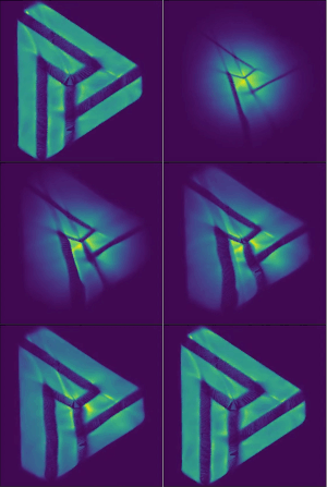
Right, so what is this GIF? You guessed it: you start with a 2D Normal distribution $N(0, I)$, and transform that smoothly into our Papercup logo — pretty cool, right? Well, we’re going to teach you how to do this with any image.

In part 1, we used normalizing flows to apply a sequence of invertible transformations to points drawn from a 2-dimensional $N(0, I)$, which transformed these points into a distribution of our choice (in that case, it was the noisy two moons distribution from sklearn). We even linked a PyTorch notebook which trained such a sequence of invertible transformations.

While we made a GIF out of it, these were really just a discrete sequence of transformations. What we did to animate it was to first obtain the sequence of sets of points: $S_0, S_1, …, S_T$ where $S_0$ are the points drawn from the $N(0, I)$ distribution, $S_T$ are the final outputs and the intermediary $S_i$’s are the outputs of layer $i$. To get the “transition” between $S_i$ and $S_{i+1}$, we simply interpolated linearly.

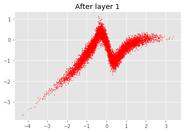
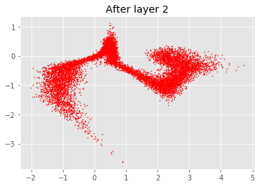
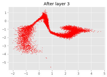
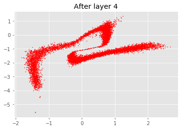
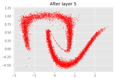
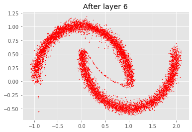
To illustrate this point, let’s plot these sets from part 1 of the tutorial, with $T=6$.

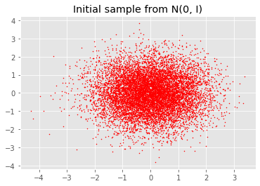
Each point from the plot at $t=0$ gets mapped to a point in the plot at $t=1$ and so on until $t=6$. To make the GIF from part 1, we simply interpolate linearly between these points.

In order to build up to making a GIF like the one above, we will first introduce Neural Ordinary Differential Equations. This was a concept introduced at NeurIPS 2018, for which the authors won best paper. Now, what are Neural ODEs? This blog post explains it well.

In short, this breakthrough is about noticing that the mathematical formulation for a very common module used in modern deep learning architectures (the residual block), is identical to the mathematical formulation of the solution to a carefully designed Ordinary Differential Equation. This means that you can replace a sequence of residual blocks by an ODE solver (which have been a very active area of research for a long time now). The paper introduces this idea and figures out the details like the training routine, etc. If you’re on the lookout for a good paper to read, I strongly recommend this one!

Ok but I still haven’t said what the point of replacing the sequence of residual blocks by an ODE solver is. Let’s get to it. What does an ODE solver allow you to do? Well, given initial conditions and an amount of time, you can follow the dynamical system defined by the ODE to solve for the position. Remember high school? If I throw a ball with a specific set of initial conditions — weight of the ball, wind, initial velocity — and an amount of time, say 3 seconds, I know what the position of the ball is (hint: it follows a parabola). Makes sense, right?

Now, in the setting described before, the “initial conditions” typically considered in an ODE solver are the inputs to the sequence of residual blocks. The “position” is the output of the sequence of residual blocks for a specific time $T$ = number of successive residual blocks. But we don’t have to only feed in $T$ to the ODE sovler ; we could feed in any number between $0$ and $T$ to get the “position” of the dynamical system at that time step. So if you feed in $t = 1$, you get the output of the first residual block, $t = 2$ the output of the second, etc. But with ODE solvers, time is not discrete, it is actually continuous. The ODE solver is actually a “generalisation” of the residual blocks, where you can get the output of “layer 1.5” in the sequence of blocks. See where the continuity of the above GIF comes from? Take a look a this image from the paper (in their case $T = 5$). You can see that on the left-hand side (traditional way of using residual blocks), you can get the output (the black circles) only at discrete layers. On the right hand side though, you can take any $t \in [0, T]$ and get a corresponding output (also the black circles). Don’t get too distracted by the arrows, they simply represent the dynamics of the system.

Okay, so that’s Neural Ordinary Differential Equations. In short, what they allow us to do is compute the output of “non-integer layers”, whatever that means. Do you see where I’m going with this? What we are going to do is apply this technique to the flows described in part 1 in order to not only be able to take the output of the $n$th layer of invertible transformations ($n$ being an integer), but also of any number in $[0, T]$, where we will define $T$ as the number of invertible transformations. The only requirement is to define the invertible transformations in a way that can be shaped like a residual block.

Well, when I said “we”, I really meant the team behind the Neural ODEs paper. Their paper is rather creatively named FFJORD: Free-Form Continuous Dynamics for Scalable Reversible Generative Models and they generously share the corresponding code here. If you go to this github link, and scroll down, you will now get an idea of how we created the GIF showed at the top. All you need to reproduce the GitHub GIF is:

• Clone the repo.
• Run python train_img2d.py --img imgs/github.png --save github_flow

You can also use your own image (we found that it worked best if the image was in black and white, where the black is the shape that you want to reproduce). Happy GIFfing, Flo Ridas.

Ok, we all like a good GIF, but what is the point? For the sake of brevity, let me try to describe this at a high level. Remember how in part 1, we had to define the invertible transformations in a way where the Jacobian was upper (or lower) triangular? This was necessary so that the determinant (used to compute the likelihood and hence the loss) was tractable. If you know a little bit about Jacobians, you will remember that they specify the change of volume factor of the transformation (and hence change of variables) to which they’re associated.

Now, in ODEs, we describe a transformation by infinitesimal change (this is how ODEs are defined). Because of that, we don’t care about the off-diagonal entries of the Jacobians! For those of you a bit baffled by this change of gears remember that for integrals, an infinitesimal change meant that the additional bit of area under the curve could be approximated by a rectangle? And this approximation enabled you to come up with (relatively) clean formulae for the integral. This is the same principle!!).

What this means, is that our choice of invertible transformations is suddenly much wider… which in turn means that we can model more interesting (invertible) transformations… which then means more data can be transformed in a more interesting manner via a flow… which, finally, means potentially more modelling power! (And, of course, even cooler GIFs)